Comprehensive Analysis of Filtering Algorithms in Machine Vision: Characteristics, Principles, and Applications

Comprehensive Analysis of Filtering Algorithms in Machine Vision: Characteristics, Principles, and Applications

Introduction

In machine vision systems, image quality directly affects the accuracy and reliability of subsequent processing tasks. During image acquisition, transmission, and storage, images inevitably suffer from various types of noise contamination, including sensor thermal noise, quantization noise, and transmission interference. These noise sources severely degrade image quality and impact the performance of critical algorithms such as feature extraction, object recognition, and edge detection. Image filtering, as a core technology in machine vision preprocessing, aims to suppress noise while preserving useful information in images, such as edges, textures, corner points, and other important features.

Image noise can be categorized into multiple types: Gaussian noise follows a normal distribution and is commonly found in electronic devices; salt-and-pepper noise manifests as random black and white pixels, often caused by transmission errors; Poisson noise is signal-dependent and frequently occurs in low-light imaging; multiplicative noise correlates with the signal itself, such as speckle noise in coherent imaging systems. Different noise types require different filtering strategies. This article systematically and comprehensively introduces mainstream filtering algorithms in machine vision, thoroughly analyzing various filtering methods from mathematical principles, algorithm characteristics, parameter effects to practical applications.

Ⅰ.Linear Filtering Algorithms

Linear filtering represents the most classical image processing approach, characterized by output pixel values being linear combinations of input pixel values. Linear filters can be efficiently implemented through convolution operations and correspond to simple multiplication in the frequency domain, offering high computational efficiency and complete theoretical framework.

1.1 Mean Filtering

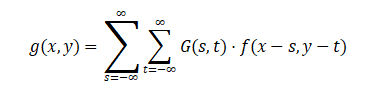
Mean filtering is the most fundamental smoothing filter, with its core concept being the replacement of the center pixel value with the arithmetic mean of all pixels within a neighborhood. The mathematical expression is:

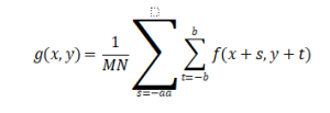
where f(x,y)represents the pixel value of the original image at coordinates(x,y) , g(x,y)is the filtered output value, the filter window size isM*N , and typically(2a+1)*(2b+1) defines the neighborhood range.

Mean filtering is essentially a low-pass filter with a frequency response of:

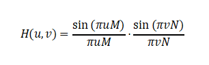
This sinc function characteristic enables mean filtering to suppress high-frequency noise while simultaneously weakening high-frequency detail information.

Algorithm Characteristics:

• Extremely simple implementation with computational complexity O(MN), can be optimized to O(1) using integral images
• Provides some suppression of additive Gaussian noise, reducing noise variance to 1/(MN) of the original
• All neighborhood pixels have equal weights, without considering spatial distance or pixel correlation
• Causes significant image blurring with severe edge sharpness degradation
• Poor performance on salt-and-pepper noise and other impulse noise types, as outliers are averaged across the entire neighborhood

Application Scenarios: Mean filtering is suitable for scenarios requiring extremely high real-time performance with less stringent image quality requirements, such as rapid preprocessing in video surveillance systems, lightweight denoising in embedded devices, and preliminary smoothing for complex algorithms. In industrial vision applications, for defect detection on uniform surfaces with minimal texture, mean filtering can serve as an initial background smoothing technique.

1.2 Gaussian Filtering

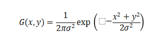
Gaussian filtering is a weighted averaging filter where weight coefficients follow a Gaussian distribution. Compared to mean filtering, Gaussian filtering assigns greater weight to the center pixel, with weights decreasing with distance, which better conforms to the statistical characteristics of natural images.

The two-dimensional Gaussian function is defined as:

The convolution operation is expressed as:

where is the standard deviation controlling the spread of the Gaussian function.

In practical applications, the Gaussian kernel is typically truncated to a or range, which contains over 99% of the energy.

Gaussian filtering possesses important mathematical properties:

• Separability: A two-dimensional Gaussian kernel can be decomposed into the product of two one-dimensional Gaussian kernels, i.e., 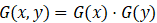, reducing computational complexity from O(N²) to O(2N)
• Rotational Invariance: The Gaussian function has circular symmetry, making filtering results independent of coordinate system choice
• Frequency Domain Characteristics: The Fourier transform of a Gaussian function remains Gaussian, which is the only function with this property

Parameter Effects: The standard deviation is the core parameter of Gaussian filtering, determining the smoothness level. Larger values produce wider Gaussian kernels with stronger smoothing effects but greater detail loss. Empirical formula: window size is typically .

Application Scenarios: Gaussian filtering is one of the most widely used smoothing filters in machine vision:

• Edge Detection Preprocessing: The Canny edge detection algorithm first uses Gaussian filtering for noise reduction to ensure gradient calculation stability
• Scale Space Construction: Feature detection algorithms like SIFT and SURF construct scale pyramids using Gaussian filtering with different values to achieve scale invariance
• Image Pyramids: In image stitching and object tracking, Gaussian pyramids provide multi-resolution representations
• Deep Learning Preprocessing: As a data augmentation technique, Gaussian blur increases model robustness
• Optical Imaging Simulation: Gaussian point spread functions simulate lens physical characteristics

1.3 Laplacian Filtering

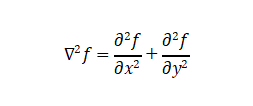
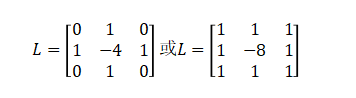
The Laplacian operator is a second-order differential operator used to detect rapid intensity changes in images, namely edges and details. The two-dimensional Laplacian operator is defined as:

Common discrete forms of the Laplacian kernel include:

Laplacian filtering is a high-pass filter that enhances high-frequency components but also amplifies noise. To address this issue, the Laplacian of Gaussian (LoG) filter is commonly employed:

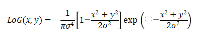
The LoG operator first smooths the image with Gaussian filtering, then calculates the Laplacian, effectively suppressing noise influence. It is widely used in blob detection, zero-crossing edge detection, image sharpening, and other applications.

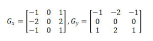
1.4 Sobel and Prewitt Operators

These are first-order derivative operators that detect edges by computing image gradients. The Sobel operator uses the following kernels:

The gradient magnitude is computed as:

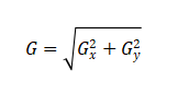
Sobel operators incorporate smoothing (through the coefficients 1, 2, 1), making them more robust to noise than simple gradient operators. They are fundamental tools in edge detection and feature extraction.

Ⅱ.Nonlinear Filtering Algorithms

While linear filtering offers theoretical completeness and computational efficiency, it suffers from inherent limitations: inability to adaptively adjust based on local image characteristics, sensitivity to impulse noise, and poor edge preservation capability. Nonlinear filtering introduces nonlinear operations to better adapt to complex image structures.

2.1 Median Filtering

     

Median filtering is a nonlinear filtering method based on order statistics, replacing the center pixel value with the median of all pixel intensities within the neighborhood:

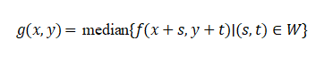
where represents the filter window and median denotes the median operation.

Algorithm Principle: The core concept of median filtering leverages the statistical property that medians are insensitive to extreme values. For a set containing n elements, the median is the element at the middle position after sorting. When isolated noise points exist in the neighborhood, these noise points are sorted to the extremes after ordering and do not affect the median selection, thus achieving noise suppression.

Algorithm Characteristics:

• Extremely strong suppression capability for salt-and-pepper (impulse) noise, maintaining good performance even with noise density up to 0.2
• Good edge sharpness preservation, as medians on both sides of an edge typically approximate the edge itself
• Less effective for Gaussian noise suppression compared to linear filters
• Higher computational complexity, with standard algorithm at O(n log n), where n is the window size
• May produce new intensity values (for even number of elements), altering the image’s intensity statistics
• Some weakening effect on fine lines and sharp corners

Improved Algorithms:

• Weighted Median Filtering: Assigns different weights (repetition counts) to pixels at different positions, with greater weight for center pixels
• Adaptive Median Filtering: Automatically adjusts window size based on noise density, formula: if Z_min<Z_med<Z_max, outputZ_med ; otherwise, increase window size
• Vector Median Filtering: For color images, considers joint statistical characteristics of RGB channels

Application Scenarios: Median filtering is widely applied in the following domains:

• Document Image Processing: Scanned documents often contain salt-and-pepper noise; median filtering effectively removes it without blurring text
• Medical Imaging: Impulse noise processing in MRI and CT images while maintaining clear lesion boundaries
• Industrial Inspection: Removing random bright and dark spots in metal surface detection while preserving defect edges
• Video Processing: Eliminating random bit errors during transmission
• Fingerprint Recognition: Preprocessing stage to remove isolated noise points while maintaining fingerprint ridge continuity

2.2 Bilateral Filtering

Bilateral filtering is a nonlinear filter that simultaneously considers spatial and range similarity, proposed by Tomasi and Manduchi in 1998. Its innovation lies in introducing intensity similarity weights to achieve edge-preserving smoothing.

The complete mathematical expression is:

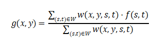
where the weight function is defined as:

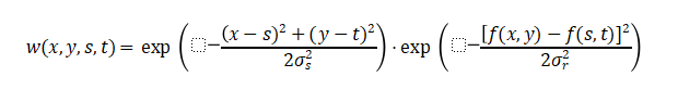
The first term G_σs is the spatial domain Gaussian kernel measuring spatial distance; the second termG_σr is the range domain Gaussian kernel measuring intensity difference.

Algorithm Principle: The key idea of bilateral filtering is that only pixels that are both spatially close and similar in intensity should participate in smoothing. In uniform regions, neighborhood pixels have similar intensities, range weights approach 1, and smoothing similar to Gaussian filtering is performed; in edge regions, pixels on opposite sides of edges have large intensity differences, range weights approach 0, mutual smoothing is suppressed, thereby preserving edge sharpness.

Parameter Effects:

• σ_s(spatial domain standard deviation): Controls spatial neighborhood size; larger values lead to broader smoothing range
• σ_r(range domain standard deviation): Controls intensity similarity threshold; larger values allow more pixels to participate in smoothing, reducing edge preservation capability
• Typical values:σ_sranges from 3-10 pixels,σ_rranges from 10%-20% of image intensity range

Algorithm Characteristics:

• Excellent edge preservation capability, known as the representative algorithm for “edge-preserving filtering”
• Good suppression of Gaussian noise and low-amplitude noise
• High computational complexity, with standard implementation at O(N²r²), where N is image size and r is filter radius
• Nonlinear operations make frequency domain analysis difficult
• Parameter selection is quite sensitive, requiring adjustment based on specific applications
• May produce “staircasing artifacts” under strong noise conditions

Acceleration Algorithms:

• Fast Bilateral Filtering: Utilizes signal processing techniques to reduce complexity to O(N)
• Bilateral Grid: Performs filtering in downsampled 3D space (x, y, intensity)
• Guided Filtering: An efficient approximation of bilateral filtering with O(N) complexity independent of window size

Application Scenarios:

• HDR Imaging: Tone mapping while preserving scene details and edges
• Image Fusion: Multi-focus image fusion, maintaining clear region boundaries
• Depth Map Processing: Depth map smoothing while preserving object boundaries
• Portrait Beautification: Skin smoothing while preserving facial contours
• Stereo Matching: Disparity map refinement, preserving depth discontinuities
• Dehazing Algorithms: Soft matting step in dark channel prior methods

2.3 Morphological Filtering

Mathematical morphology is an image analysis method based on set theory, extracting image features through interactions between structuring elements and images. Basic morphological operations include erosion and dilation.

Erosion is defined as:

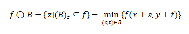
Dilation is defined as:

whereis the structuring element and is the reflection of .

Based on erosion and dilation, more complex morphological operations can be defined:

Opening: Erosion followed by dilation

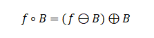
Opening can eliminate small bright regions, smooth object contours, and break thin connections.

Closing: Dilation followed by erosion

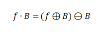
Closing can fill small dark regions, connect adjacent objects, and fill thin cracks.

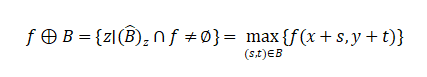
Morphological Gradient:

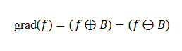
Morphological gradient extracts object edges and is more robust compared to traditional gradient operators.

Top-hat Transform:

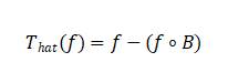
Extracts bright features smaller than the structuring element.

Black-hat Transform:

Extracts dark features smaller than the structuring element.

Structuring Element Design: The shape and size of the structuring element determine the effect of morphological operations:

• Square: Isotropic, suitable for general purposes
• Circular: Rotation invariant, suitable for features without directionality
• Linear: Detects structures in specific directions
• Cross-shaped: Preserves connectivity

Application Scenarios:

• Binary Image Processing: Removing noise points, filling holes, extracting skeletons
• OCR Preprocessing: Character segmentation, stroke repair
• Industrial Inspection: Surface defect detection, particle analysis, dimension measurement
• Biomedical Applications: Cell counting, tissue segmentation
• Document Analysis: Layout analysis, table extraction
• Traffic Monitoring: Vehicle extraction, license plate localization

2.4 Anisotropic Diffusion Filtering

Anisotropic diffusion, proposed by Perona and Malik, is a partial differential equation (PDE) driven filtering method. Its basic idea is to adaptively adjust diffusion intensity based on local image gradients, performing isotropic diffusion in uniform regions while suppressing diffusion perpendicular to edge directions in edge regions.

The partial differential equation is expressed as:

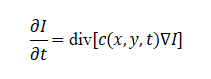
where is the image, is evolution time, is the divergence operator, is the gradient operator, and c(x,y,t)is the diffusion coefficient.

The diffusion coefficient is typically defined as a decreasing function of gradient:

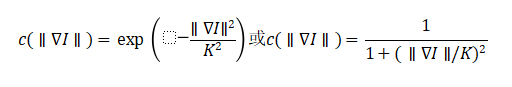
where is a threshold parameter controlling edge strength.

Algorithm Characteristics:

• Sharpens edges while smoothing images, achieving “edge-sharpening denoising”
• Can handle complex edge structures and textures
• Relatively complex computation requiring iterative PDE solution
• Parameter selection is critical, requiring balance between denoising and edge preservation

Applications: Medical image enhancement, remote sensing image processing, artistic stylization, etc.

2.5 Total Variation Filtering

Total Variation (TV) filtering is based on the principle that natural images have sparse gradients. It minimizes the total variation while fitting the observed data:

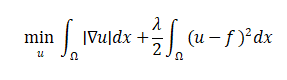
where is the restored image, is the noisy observation, and is the regularization parameter.

TV filtering excels at preserving edges while removing noise, but can produce staircasing artifacts in smooth gradient regions. It is particularly effective for piecewise constant images and is widely used in compressed sensing, image reconstruction, and denoising applications.

III. Frequency Domain Filtering Algorithms

Frequency domain filtering is based on Fourier transform theory, processing images in the frequency domain. According to the convolution theorem, spatial domain convolution equals frequency domain multiplication, providing a new perspective for understanding and designing filters.

Fourier Transform:

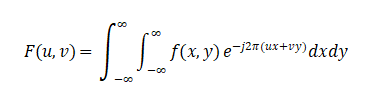
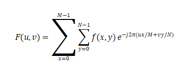
Discrete form (DFT):

3.1 Low-Pass Filters

Low-pass filters allow low-frequency components to pass while suppressing high-frequency components, achieving image smoothing.

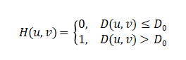
Ideal Low-Pass Filter (ILPF):

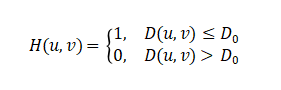
where is the distance from the frequency point to the center, and is the cutoff frequency.

The ideal low-pass filter has sharp frequency cutoff characteristics but produces obvious ringing effects in the spatial domain because its spatial response is a sinc function with infinite spatial support.

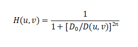
Butterworth Low-Pass Filter (BLPF):

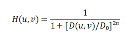
where is the filter order. The Butterworth filter provides smooth transition between passband and stopband. When n=1 , ringing effects are minimal; as n increases, it gradually approaches the ideal filter.

Gaussian Low-Pass Filter (GLPF):

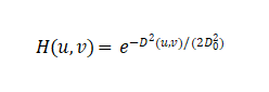
The Gaussian low-pass filter has no ringing effects because the Fourier transform of a Gaussian function remains Gaussian, with smooth and spatially localized spatial response.

3.2 High-Pass Filters

High-pass filters suppress low-frequency components while preserving high-frequency components, used for edge enhancement and sharpening. High-pass filters can be derived from low-pass filters through .

The three main types mirror their low-pass counterparts:

Ideal High-Pass Filter (IHPF):

Butterworth High-Pass Filter (BHPF):

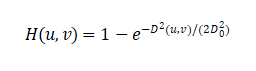
Gaussian High-Pass Filter (GHPF):

Applications: Edge extraction, image sharpening, texture analysis, unsharp masking for detail enhancement.

3.3 Band-Pass and Band-Stop Filters

Band-pass filters allow specific frequency ranges to pass, used for extracting specific frequency textures or periodic patterns. Band-stop filters (notch filters) suppress specific frequencies, commonly used for removing periodic noise such as scanning line interference and moiré patterns.

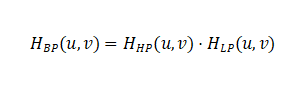
Band-Pass Filter:

Band-Stop Filter:

Notch Filter: Specifically designed to reject narrow frequency bands, typically used to eliminate periodic interference at known frequencies. The transfer function is:

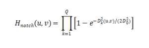
where is the distance to the -th notch center.

Selective Filtering Applications:

• Removing power line interference (50Hz/60Hz harmonics)
• Eliminating printing halftone dot patterns
• Removing periodic texture interference in fabric inspection
• Suppressing scan line artifacts in video

3.4 Homomorphic Filtering

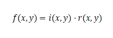
Homomorphic filtering operates in the frequency domain to simultaneously normalize illumination and enhance contrast. It exploits the fact that images can be modeled as the product of illumination and reflectance:

Taking logarithm converts multiplication to addition:

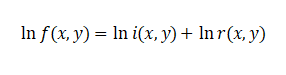
After Fourier transform, different frequency filters are applied to illumination (low frequency) and reflectance (high frequency) components, followed by inverse transform and exponentiation.

Applications: Correcting non-uniform illumination, enhancing details in shadowed regions, medical X-ray enhancement, underwater image restoration.

IV.Adaptive Filtering Algorithms

Adaptive filters can automatically adjust filtering parameters based on local statistical characteristics of images, employing different processing strategies in different regions to achieve more intelligent noise suppression.

4.1 Wiener Filtering

Wiener filtering is the optimal linear filter that restores degraded images under the minimum mean square error (MMSE) criterion. The frequency domain expression is:

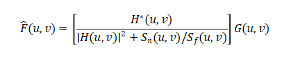
where H(u,v) is the degradation function, S_n and  S_f  are the power spectra of noise and original signal respectively, G(u,v) and is the spectrum of the degraded image.

When the signal-to-noise ratio is very high (S_n/S_f→0), Wiener filtering degrades to the inverse filter 1/H; when the signal-to-noise ratio is very low, Wiener filtering performs stronger smoothing. This adaptive characteristic makes it perform excellently in image restoration, deblurring, and other applications.

Simplified Wiener Filter: When the power spectra are unknown, a constant noise-to-signal ratio K can be assumed:

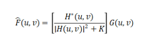
The parameter K controls the trade-off between inverse filtering and noise smoothing.

4.2 Local Adaptive Filtering

Adaptive filters based on local statistical characteristics adjust filtering intensity according to neighborhood variance:

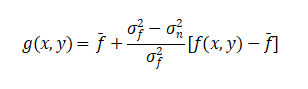
where is the local mean, is the local variance, and is the noise variance.

Adaptive Mechanism:

• In uniform regions with small variance : Strong smoothing is applied, output approaches local mean
• In edge and texture regions with large variance : Minimal filtering, original values are preserved
• The max operation ensures non-negative weights, preventing noise amplification

Lee Filter and Frost Filter: Similar adaptive approaches used in SAR (Synthetic Aperture Radar) image processing, specifically designed for multiplicative speckle noise.

4.3 Non-Local Means Filtering

Non-Local Means (NLM) filtering exploits image self-similarity by searching the entire image for similar patches and performing weighted averaging:

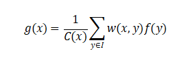
The weight is defined as:

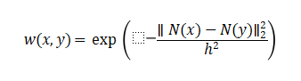
where N(x) and N(y) are image patches centered at x and y , and controls the decay rate.

Normalization Factor:

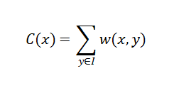
Algorithm Principle: NLM is based on the observation that natural images contain redundant information—similar structures repeat throughout the image. By averaging all similar patches rather than just local neighbors, NLM achieves superior denoising while preserving fine details.

Key Parameters:

• Patch size: Typically 5×5 or 7×7; larger patches better capture structure but increase computation
• Search window: Defines the region for finding similar patches; typical size 21×21
• Filtering parameter h: Controls weight decay; should be proportional to noise standard deviation

Computational Complexity: Standard NLM has O(N²P²) complexity, where N is image size and P is patch size. Fast implementations using integral images, PCA, or FFT can reduce this significantly.

Applications: Natural image denoising, texture preservation, MRI denoising, video denoising (exploiting temporal redundancy).

4.4 Block-Matching and 3D Filtering (BM3D)

BM3D represents the state-of-the-art in traditional denoising algorithms, combining:

1. Block-matching: Finding similar patches throughout the image
2. Collaborative filtering: Stacking similar patches into 3D groups and filtering in transform domain
3. Aggregation: Weighted averaging of all estimates

The algorithm operates in two steps:

• Step 1: Hard-thresholding in 3D transform domain to obtain basic estimate
• Step 2: Wiener filtering using the basic estimate as reference

BM3D achieves exceptional PSNR results but requires significant computation. It serves as a benchmark for evaluating learning-based methods.

V.Wavelet-Based Filtering

Wavelet transforms provide multi-scale, multi-resolution analysis, offering both time and frequency localization unlike Fourier transforms.

5.1 Discrete Wavelet Transform (DWT)

The 2D DWT decomposes an image into approximation and detail coefficients at multiple scales:

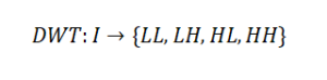
where LL contains low-frequency approximation, LH contains horizontal details, HL vertical details, and HH diagonal details.

Wavelet Denoising Procedure:

1. Decomposition: Apply DWT to noisy image
2. Thresholding: Apply threshold to detail coefficients
3. Reconstruction: Inverse DWT to obtain denoised image

Thresholding Methods:

Hard Thresholding:

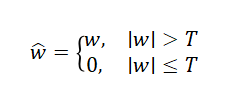
Soft Thresholding:

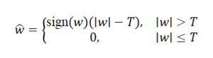
where T is the threshold, often set as (universal threshold), with σ being noise standard deviation.

Advantages:

• Sparse representation of natural images
• Good edge preservation
• Effective for various noise types
• Multi-resolution analysis capability

Common Wavelets: Haar, Daubechies (db), Symlets, Coiflets, Biorthogonal

Applications: Medical image denoising, compression, texture analysis, feature extraction for classification.

VI. Deep Learning-Based Denoising Methods

In recent years, deep learning-based image denoising methods have achieved breakthrough progress, surpassing the performance limits of traditional filtering algorithms.

6.1 Convolutional Neural Network Denoising

DnCNN (Denoising CNN):

• Learns residual noise mapping:R(y)=y−x , where y is noisy, x is clean
• Uses batch normalization and residual learning
• Single model handles various noise levels
• Architecture: 17-20 convolutional layers with ReLU activations

FFDNet (Fast and Flexible Denoising Network):

• Non-blind denoising with noise level map as input
• Downsampling for computational efficiency
• Orthogonal regularization for feature diversity
• Better balance between speed and quality

**Noise2Noise**: Revolutionary approach training on pairs of noisy images without clean targets:

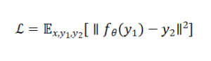
where y1,y2 are independent noisy observations of x.

6.2 Generative Adversarial Networks

GANs generate more realistic textures and details, avoiding over-smoothing characteristic of MSE-based methods.

Architecture:

• Generator: Transforms noisy input to clean output
• Discriminator: Distinguishes real clean images from generated ones
• Perceptual Loss: Uses pre-trained VGG features for better perceptual quality

Advantages: Superior visual quality, realistic texture synthesis, better for high-noise scenarios

Challenges: Training instability, mode collapse, longer convergence time

6.3 Attention Mechanisms

Attention modules help networks focus on important regions, improving edge and detail recovery quality.

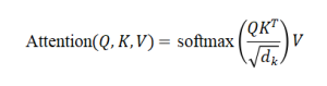
Self-Attention:

Channel Attention: Squeezes spatial information and emphasizes important feature channels (e.g., Squeeze-and-Excitation blocks)

Spatial Attention: Highlights important spatial locations

Non-Local Neural Networks: Compute responses at a position as weighted sum of features at all positions, capturing long-range dependencies similar to NLM but learned end-to-end.

6.4 Transformer-Based Denoising

Vision Transformers and their variants (Swin Transformer, Restormer) have been adapted for image denoising:

• Global receptive field through self-attention
• Better long-range dependency modeling
• State-of-the-art results on benchmark datasets
• Higher computational cost than CNNs

Restormer: Combines transformers with convolutional features, achieving excellent performance on multiple restoration tasks including denoising, deraining, and deblurring.

VII. Filtering Algorithm Selection Strategy

Selecting appropriate filtering algorithms in practical applications requires comprehensive consideration of multiple factors:

7.1 Noise Type Considerations

Gaussian Noise:

• First choice: Gaussian filtering, Wiener filtering, BM3D
• Deep learning: DnCNN, FFDNet
• Balance: Bilateral filtering for edge preservation

Salt-and-Pepper (Impulse) Noise:

• Best: Median filtering, adaptive median filtering
• Morphological filters for binary images
• Avoid: Linear filters (spread noise)

Poisson Noise (Signal-Dependent):

• Anscombe transform + Gaussian noise methods
• Specialized Poisson denoising algorithms
• Deep learning trained on Poisson noise

Speckle Noise (Multiplicative):

• Lee filter, Frost filter for SAR images
• Logarithmic transform + additive noise methods
• Wavelet-based approaches

Periodic Noise:

• Frequency domain notch filtering
• Band-stop filters
• Comb filters for specific patterns

7.2 Edge Preservation Requirements

High Priority Edge Preservation:

• Bilateral filtering
• Anisotropic diffusion
• Guided filtering
• Total variation methods
• Deep learning (trained with perceptual loss)

Moderate Edge Preservation:

• Gaussian filtering (small σ)
• Adaptive filters
• Wavelet soft thresholding

Edge Enhancement Acceptable:

• Morphological operations
• Median filtering
• Unsharp masking

7.3 Computational Resource Constraints

Real-Time Systems (< 30ms per frame):

• Mean filtering (integral image optimization)
• Fast bilateral approximations
• Separable filters
• GPU-accelerated deep learning inference

Embedded Devices (Limited Memory/Power):

• Simple linear filters
• Median filtering (optimized)
• Lightweight neural networks (MobileNet-based)

Offline Processing (Quality Priority):

• BM3D
• Non-local means
• Large deep learning models
• Iterative optimization methods

7.4 Image Characteristics

Texture-Rich Images:

• Non-local means
• Wavelet methods
• Texture-preserving GANs
• Avoid: Strong smoothing filters

Simple Structures:

• Gaussian filtering
• Basic morphological operations
• Lightweight methods sufficient

Medical Images (High Fidelity Required):

• Conservative filtering
• Wavelet methods
• Anisotropic diffusion
• Careful parameter tuning
• Validation by medical professionals

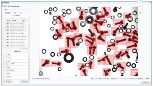
Industrial Inspection (Robustness Priority):

• Robust to illumination changes
• Morphological processing
• Adaptive thresholding
• Ensemble approaches

7.5 Application Domain Specific

Autonomous Driving:

• Real-time requirement critical
• Weather/lighting robustness
• GPU acceleration essential
• Temporal consistency (video)

Medical Imaging:

• Diagnostic quality paramount
• FDA/CE approval considerations
• Reproducibility required
• Conservative approaches preferred

Surveillance:

• 24/7 operation
• Variable lighting conditions
• Low-light performance
• Compression artifact handling

Scientific Imaging:

• Quantitative accuracy
• Minimal bias introduction
• Reversible operations preferred
• Statistical characterization needed

7.6 Hybrid Approaches

Modern systems often combine multiple filtering methods:

Pipeline Example 1 (General Preprocessing):

1. Gaussian filtering (initial noise reduction)
2. Bilateral filtering (edge-preserving smoothing)
3. Morphological operations (feature extraction)

Pipeline Example 2 (Medical Imaging):

1. Anisotropic diffusion (structure preservation)
2. Wavelet thresholding (detail recovery)
3. Adaptive histogram equalization (contrast enhancement)

Pipeline Example 3 (Industrial Vision):

1. Median filtering (impulse noise removal)
2. Morphological closing (hole filling)
3. Edge detection with hysteresis

Learning-Based Hybrid:

1. Traditional filtering (fast initial denoising)
2. Deep network (refinement stage)
3. Post-processing (artifact removal)

VIII. Evaluation Metrics

Quantifying filtering performance requires appropriate metrics:

8.1 Objective Metrics (With Reference)

Peak Signal-to-Noise Ratio (PSNR):

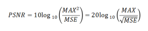
where

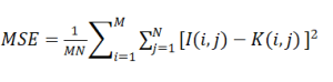
Higher values indicate better quality, but doesn’t always correlate with perceptual quality.

Structural Similarity Index (SSIM):

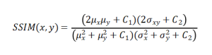
Considers luminance, contrast, and structure; better perceptual correlation than PSNR.

Mean Absolute Error (MAE):

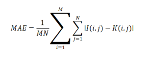
More robust to outliers than MSE.

8.2 Perceptual Metrics

Learned Perceptual Image Patch Similarity (LPIPS): Uses deep features from pre-trained networks; better aligns with human perception than traditional metrics.

Natural Image Quality Evaluator (NIQE): No-reference metric based on natural scene statistics.

8.3 Task-Specific Metrics

Edge Preservation Index: Measures how well edges are maintained after filtering.

Computational Time: Critical for real-time applications

Memory Footprint: Important for embedded systems

IX.Future Trends and Emerging Directions

9.1 Self-Supervised and Unsupervised Learning

Noise2Void: Learns denoising without clean images by predicting center pixel from surrounding context.

Blind-Spot Networks: Ensures network doesn’t use the noisy pixel itself, preventing identity mapping.

9.2 Physics-Informed Neural Networks

Combining physical image formation models with deep learning for interpretable and generalizable denoising.

9.3 Few-Shot and Meta-Learning

Adapting to new noise types with minimal training data.

9.4 Real-Time Deep Learning

Neural Architecture Search (NAS): Automatically designing efficient networks

Knowledge Distillation: Compressing large models to lightweight versions

Quantization: Reducing precision while maintaining performance

9.5 Explainable AI in Filtering

Understanding what deep networks learn and ensuring safety-critical applications can trust the results.

X. Conclusion

Machine vision filtering algorithms have evolved from simple linear filters to complex adaptive methods and now to learning-based intelligent filters. Each algorithm possesses unique advantages and application scenarios—no single algorithm can solve all problems. Understanding these algorithms’ mathematical principles, characteristics, and applications is fundamental to building high-performance machine vision systems.

Modern machine vision systems often employ combinations of multiple filtering algorithms: initial Gaussian filtering for preliminary smoothing, followed by bilateral filtering for edge-preserving denoising, and finally morphological operations for feature extraction. With increasing computational power and advancing deep learning technology, learning-based filters are becoming research hotspots, capable of automatically learning optimal filtering strategies adapted to various complex scenarios.

However, traditional filtering algorithms remain indispensable in many applications due to their theoretical completeness, interpretability, and computational efficiency. The future of image filtering lies not in replacing traditional methods with deep learning, but in intelligently combining both approaches: leveraging traditional filters’ efficiency and reliability for preprocessing while employing deep learning for complex, high-level denoising tasks. This hybrid paradigm, coupled with domain-specific knowledge and application requirements, will continue driving innovation in machine vision technology.

As imaging technology advances—with higher resolutions, new sensor modalities (hyperspectral, light field, computational imaging), and emerging applications (AR/VR, autonomous systems, space exploration)—filtering algorithms must continue evolving. The next generation of filters will likely be adaptive not just to local image statistics, but to semantic content, task requirements, and even user preferences, ushering in an era of truly intelligent image processing.